note: this tutorial is loosely based off the DESeq2 and bioconductor documentation found here. Some explanation text is taken directly from the documentation and referenced.

In this tutorial, we will walk through going from gene counts to differential expression results.

Introduction

The true end goal in RNA Sequencing analysis is determining the genes that are differentially expressed between a control and treatment group. In this case, if you followed the previous tutorial, you know we are investigating the transcriptomic response of TCPMOH on the developing zebrafish. In this dataset subset we have two control biological replicates and two TCPMOH biological replicates. To perform differential expression analysis, we will be using using DESeq2 (Love, Huber, and Anders 2014). DESeq2 is a great tool for dealing with RNA-seq data and running Differential Gene Expression (DGE) analysis. It takes read count files from different samples, combines them into a big table (with genes in the rows and samples in the columns) and applies normalization for sequencing depth and library composition. We do not need to account for gene length normalization does because we are comparing the counts between sample groups for the same gene.

Load necessary packages

The first step is to make sure we have the proper packages loaded. We will be using DESeq2, tidyverse, and ggplot2. If you haven’t already installed these before, you can run the following commands:

# install DESeq2
if (!require("BiocManager", quietly = TRUE))
    install.packages("BiocManager")

BiocManager::install("DESeq2")

# install tidyverse (ggplot2 is in tidyverse)
install.packages("tidyverse")

Now we can load the packages into our workspace by running the following commands:

# package setup
library( "DESeq2" )
library(tidyverse)
library(ggplot2)

Getting Started - Data

This tutorial assumes you have a file, per sample, of gene counts. This would be a typical output from a tool such as featureCounts which we used in the previous tutorial. To give an idea of what this looks like, lets peak into one of the files:

# define the path to the file
# note this path is relative to the current working directory and the files are stored in a folder called data
dmso1_data_file_path <- 'data/DMSO_1_counts.tsv'
# read in the file
dmso_1_count_data <- read.csv(dmso1_data_file_path, header = TRUE, sep = "\t")
# show the first few lines
head(dmso_1_count_data)

##   Geneid DMSO_1.RNA.STAR..mapped.bam
## 1   CYTB                      136445
## 2    ND6                        1443
## 3    ND5                       77429
## 4    ND4                       71269
## 5   ND4L                       12122
## 6    ND3                       10141

As you can see, the file has two columns. One identifying the gene name (Geneid) and the second identifying the number of counts per gene. It is useful to go ahead and rename the second column as it is currently cumbersome.

# rename the second column
colnames(dmso_1_count_data)[2] ="DMSO_1"

Lets go ahead and do this for the rest of the samples:

# dmso2
dmso_2_count_data <- read.csv('data/DMSO_2_counts.tsv', header = TRUE, sep = "\t")
colnames(dmso_2_count_data)[2] ="DMSO_2"

# tcpmoh1
tcpmoh_1_count_data <- read.csv('data/TCPMOH_1_counts.tsv', header = TRUE, sep = "\t")
colnames(tcpmoh_1_count_data)[2] ="TCPMOH_1"

# tcpmoh2
tcpmoh_2_count_data <- read.csv('data/TCPMOH_2_counts.tsv', header = TRUE, sep = "\t")
colnames(tcpmoh_2_count_data)[2] ="TCPMOH_2"

Organize Data

To actually run DESeq2, we want all the gene count data in one data frame. Therefore, we need to merge the data sets based on the Geneid.

# put all data frames into list
df_list <- list(dmso_1_count_data, dmso_2_count_data, tcpmoh_1_count_data, tcpmoh_2_count_data)

# merge all data frames in list
count_data <- df_list %>% reduce(full_join, by='Geneid')
# make the Geneid the row id 
count_data <- count_data %>% remove_rownames %>% column_to_rownames(var="Geneid")
head(count_data)

##      DMSO_1 DMSO_2 TCPMOH_1 TCPMOH_2
## CYTB 136445 176209   137586   193845
## ND6    1443   2208     1317     1695
## ND5   77429  93110    74762    93454
## ND4   71269  94885    79189   100194
## ND4L  12122  14628    11453    14168
## ND3   10141  14687    10184    13766

We also need a meta data table. This can be done in R or by filling out a csv/tsv file and reading it in. I will just generate it here.

# get the sample names from the count_data matrix
SampleName <- c(colnames(count_data))
# specify the conditions for each sample
# In my sample names, DMSO_1 and DMSO_2 are control replicated and TCPMOH_1 and TCPMOH_2 are treated replicates
condition <- c("control", "control", "treated", "treated")
# generate the metadata data frame
meta_data <- data.frame(SampleName, condition)
# make the sample name the row id
meta_data <- meta_data %>% remove_rownames %>% column_to_rownames(var="SampleName")
meta_data

##          condition
## DMSO_1     control
## DMSO_2     control
## TCPMOH_1   treated
## TCPMOH_2   treated

We want to double check that the name of the columns in the counts matrix is the same as the names in the meta data file. We can do this using the following two lines of code. Ideally, you should see TRUE and TRUE returned. If not, the rows in meta_data do not match the columns in counts_data and you should trouble shoot before moving forward. This is usually just a misorganization somewhere or a typo.

all(colnames(count_data) %in% rownames(meta_data))

## [1] TRUE

all(colnames(count_data) == rownames(meta_data))

## [1] TRUE

Differential Expression Analysis

Set Up DESeq Objects

Now that we have the data organized, we can run the differential expression analysis. The first step is to create a DESeq data object to complete the downstream analysis.

# create deseq data set object
dds <- DESeqDataSetFromMatrix(countData = count_data,
                              colData = meta_data,
                              design = ~ condition)

We can investigate the DESeq object:

# run the below to see the object elements
dds

## class: DESeqDataSet 
## dim: 30421 4 
## metadata(1): version
## assays(1): counts
## rownames(30421): CYTB ND6 ... cep97 rpl24
## rowData names(0):
## colnames(4): DMSO_1 DMSO_2 TCPMOH_1 TCPMOH_2
## colData names(1): condition

We see here that the dimension is 36351x4 meaning we have 36351 genes and 4 samples. The row names are the gene ids. Everything looks as it should! An optional step is to pre fliter some of the genes with low counts.

Pre-Filtering

While it is not necessary to pre-filter low count genes before running the DESeq2 functions, there are two reasons which make pre-filtering useful: by removing rows in which there are very few reads, we reduce the memory size of the dds data object, and we increase the speed of the transformation and testing functions within DESeq2. It can also improve visualizations, as features with no information for differential expression are not plotted.

# filter any counts less than 10
keep <- rowSums(counts(dds)) >= 10
dds <- dds[keep,]
dds

## class: DESeqDataSet 
## dim: 24356 4 
## metadata(1): version
## assays(1): counts
## rownames(24356): CYTB ND6 ... cep97 rpl24
## rowData names(0):
## colnames(4): DMSO_1 DMSO_2 TCPMOH_1 TCPMOH_2
## colData names(1): condition

You can see that when we pre-filter, we end up with 26859 genes left. The only downside to this step is these genes will no longer be included in the final output file. This isn’t an issue for most cases but if you are like me and often aggregate results from multiple studies, this can make your life difficult as the number of genes will now be different. Anyway, pre-filtering is great if you are just running a ‘typical’ workflow.

Set Reference Factor

By default, R will choose a reference level for factors based on alphabetical order. Then, if you never tell the DESeq2 functions which level you want to compare against (e.g. which level represents the control group), the comparisons will be based on the alphabetical order of the levels. Here, we just want to be sure the level we are comparing against is truly the control using the relevel function.

# set the reference to be the control
dds$condition <- relevel(dds$condition, ref = 'control')

Getting Normalized Counts

Sometimes, we want the normalized counts as an output for downstream analysis. To obtain them, you can run the following commands.

# get normalized counts
dds <- estimateSizeFactors(dds)
normalized_counts <- counts(dds, normalized = TRUE)

# If you would like to write the normalized counts to a file, you can run the following command. Note that you need to specify the file path. 
# write.table(normalized_counts, file=normalized_counts_data_file_path, sep = '\t', quote=F, col.names = NA)

Run Differential Expression

The standard differential expression analysis steps are wrapped into a single function, DESeq. Results tables are generated using the function results, which extracts a results table with log2 fold changes, p values and adjusted p values. With no additional arguments to results, the log2 fold change and Wald test p value will be for the last variable in the design formula, and if this is a factor, the comparison will be the last level of this variable over the reference level (see previous note on factor levels). However, the order of the variables of the design do not matter so long as the user specifies the comparison to build a results table for, using the name or contrast arguments of results.

dds <- DESeq(dds)
res <- results(dds)
res

## log2 fold change (MLE): condition treated vs control 
## Wald test p-value: condition treated vs control 
## DataFrame with 24356 rows and 6 columns
##          baseMean log2FoldChange     lfcSE      stat    pvalue      padj
##         <numeric>      <numeric> <numeric> <numeric> <numeric> <numeric>
## CYTB    158703.52      0.0480368  0.105504  0.455308 0.6488875  0.962519
## ND6       1643.65     -0.2958785  0.155837 -1.898644 0.0576113  0.487636
## ND5      83990.25     -0.0468041  0.102839 -0.455123 0.6490211  0.962519
## ND4      85437.84      0.0876639  0.110877  0.790639 0.4291546  0.917258
## ND4L     12990.62     -0.0880488  0.107552 -0.818662 0.4129792  0.908968
## ...           ...            ...       ...       ...       ...       ...
## hikeshi  1064.229      0.0618543  0.146767  0.421445  0.673430  0.966905
## eed       875.412     -0.0960908  0.166265 -0.577937  0.563307  0.948176
## nfkbiz    948.290      0.0612779  0.172558  0.355116  0.722503  0.977389
## cep97     661.991     -0.0895011  0.212066 -0.422043  0.672993  0.966905
## rpl24   35114.027      0.1329105  0.123686  1.074584  0.282561  0.844292

We can also get a summary:

summary(res)

## 
## out of 24356 with nonzero total read count
## adjusted p-value < 0.1
## LFC > 0 (up)       : 201, 0.83%
## LFC < 0 (down)     : 270, 1.1%
## outliers [1]       : 0, 0%
## low counts [2]     : 9916, 41%
## (mean count < 204)
## [1] see 'cooksCutoff' argument of ?results
## [2] see 'independentFiltering' argument of ?results

If you would like to know the exact number of adjusted p-values that are <0.01, you can run the following command:

sum(res$padj < 0.1, na.rm=TRUE)

## [1] 471

As you can see, the results function defaults to a p-value <0.1. For stronger statistical significance, we often want to look at those <0.05. This can be specified in the results function:

res05 <- results(dds, alpha=0.05)
summary(res05)

## 
## out of 24356 with nonzero total read count
## adjusted p-value < 0.05
## LFC > 0 (up)       : 148, 0.61%
## LFC < 0 (down)     : 197, 0.81%
## outliers [1]       : 0, 0%
## low counts [2]     : 6611, 27%
## (mean count < 75)
## [1] see 'cooksCutoff' argument of ?results
## [2] see 'independentFiltering' argument of ?results

And then the number of genes with an adjusted p-value <0.05 are:

sum(res$padj < 0.05, na.rm=TRUE)

## [1] 348

As you can see, this number is less as an adjusted p-value <0.05 is a stronger statistical significance. At this point, it is useful to download the results into one location. We can do that by writing the results to a csv file.

# write results to file, notice you need to specify the file path. 
# write.csv(as.data.frame(res), file=deseq_results_file_path)

Visualizing Results

At this point, we can visualize and make conclusions for our data. The first question is what is considered a differentially expressed gene? There are two things to consider: (1) the lof2FC value and (2) the adjusted p-value.

DESeq2 uses the so-called Benjamini-Hochberg (BH) adjustment; in brief, this method calculates for each gene an adjusted p value which answers the following question: if one called significant all genes with a p value less than or equal to this gene’s p value threshold, what would be the fraction of false positives (the false discovery rate, FDR) among them (in the sense of the calculation outlined above)? These values, called the BH-adjusted p values, are given in the column padj of the results object. Hence, if we consider a fraction of 10% false positives acceptable, we can consider all genes with an adjusted p value below 10%=0.1 as significant.

Mathematically speaking, any log2FC value different than zero with low variability. Typically speaking, you will see people identify a differentially expressed gene for log2FC cutoff value between 1-1.5 (positive or negative). Additionally, the adjusted p-value is typically chosen to be <0.05 but is sometimes chosen to be <0.1 (DESeq default) or even <0.01 for stronger statistical confidence. For this tutorial, I will choose genes with an adjusted p-value <0.05 and a |Log2FC|<1.

# convert results data to basic dataframe
data <- data.frame(res)
head(data)

##        baseMean log2FoldChange     lfcSE       stat     pvalue      padj
## CYTB 158703.518     0.04803679 0.1055039  0.4553082 0.64888750 0.9625189
## ND6    1643.651    -0.29587855 0.1558368 -1.8986437 0.05761133 0.4876364
## ND5   83990.255    -0.04680413 0.1028385 -0.4551225 0.64902109 0.9625189
## ND4   85437.841     0.08766391 0.1108773  0.7906391 0.42915461 0.9172576
## ND4L  12990.616    -0.08804881 0.1075521 -0.8186621 0.41297922 0.9089675
## ND3   12017.929    -0.07758008 0.1247725 -0.6217724 0.53409151 0.9438768

Notice the column names! The columns we are typically interested in are log2FoldChange and padj.

PCA Plot

Portions of this section were taken from this tutorial. DESeq2 has a built-in function for plotting PCA plots, that uses ggplot2 under the hood. This is great because it saves us having to type out lines of code and having to fiddle with the different ggplot2 layers. In addition, it takes the rlog object as an input directly, hence saving us the trouble of extracting the relevant information from it.

The function plotPCA() requires two arguments as input: an rlog object and the intgroup (the column in our metadata that we are interested in).

rld <- rlog(dds)
plotPCA(rld)

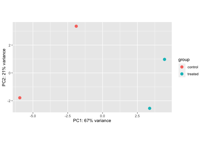
By default the function uses the top 500 most variable genes. Ideally, we would want to see that our samples cluster together based on treatment group.

Volcano Plots

A volcano plot is a type of scatterplot that shows statistical significance (P value) versus magnitude of change (fold change). It enables quick visual identification of genes with large fold changes that are also statistically significant. These may be the most biologically significant genes. We can get as simple or as fancy as we would like when it comes to volcano plots!

Identify Up and Down Regulated Genes

# add an additional column that identifies a gene as unregulated, downregulated, or unchanged
# note the choice of pvalue and log2FoldChange cutoff. 
data <- data %>%
  mutate(
  Expression = case_when(log2FoldChange >= log(1) & padj <= 0.05 ~ "Up-regulated",
  log2FoldChange <= -log(1) & padj <= 0.05 ~ "Down-regulated",
  TRUE ~ "Unchanged")
  )
head(data)

##        baseMean log2FoldChange     lfcSE       stat     pvalue      padj
## CYTB 158703.518     0.04803679 0.1055039  0.4553082 0.64888750 0.9625189
## ND6    1643.651    -0.29587855 0.1558368 -1.8986437 0.05761133 0.4876364
## ND5   83990.255    -0.04680413 0.1028385 -0.4551225 0.64902109 0.9625189
## ND4   85437.841     0.08766391 0.1108773  0.7906391 0.42915461 0.9172576
## ND4L  12990.616    -0.08804881 0.1075521 -0.8186621 0.41297922 0.9089675
## ND3   12017.929    -0.07758008 0.1247725 -0.6217724 0.53409151 0.9438768
##      Expression
## CYTB  Unchanged
## ND6   Unchanged
## ND5   Unchanged
## ND4   Unchanged
## ND4L  Unchanged
## ND3   Unchanged

Get the Top 10 Most Variable Genes

top <- 10
# we are getting the top 10 up and down regulated genes by filtering the column Up-regulated and Down-regulated and sorting by the adjusted p-value. 
top_genes <- bind_rows(
  data %>%
  filter(Expression == 'Up-regulated') %>%
  arrange(padj, desc(abs(log2FoldChange))) %>%
  head(top),
  data %>%
  filter(Expression == 'Down-regulated') %>%
  arrange(padj, desc(abs(log2FoldChange))) %>%
  head(top)
  )
# create a datframe just holding the top 10 genes
Top_Hits = head(arrange(data,pvalue),10)
Top_Hits

##                    baseMean log2FoldChange     lfcSE      stat       pvalue
## pdk2b             9748.7672       1.329178 0.1346152  9.873903 5.402079e-23
## si:ch211-132b12.7 4790.7498      -1.239026 0.1256370 -9.861952 6.085478e-23
## trim63a            622.7489       1.887092 0.1942775  9.713383 2.644124e-22
## eevs              2600.6421      -1.623744 0.1680947 -9.659699 4.471781e-22
## zgc:113054        3347.4297      -1.115578 0.1315768 -8.478527 2.280618e-17
## si:ch211-161h7.5  2632.1364      -1.424045 0.1735748 -8.204213 2.321063e-16
## hebp2             2600.6605      -1.098667 0.1359765 -8.079829 6.485740e-16
## ndrg1b             716.7809       1.302238 0.1659977  7.844918 4.332367e-15
## psme4a            1946.1987       1.279067 0.1718202  7.444217 9.752090e-14
## hsp70.3            817.8511      -1.287905 0.1735650 -7.420303 1.168528e-13
##                           padj     Expression
## pdk2b             4.393715e-19   Up-regulated
## si:ch211-132b12.7 4.393715e-19 Down-regulated
## trim63a           1.272705e-18   Up-regulated
## eevs              1.614313e-18 Down-regulated
## zgc:113054        6.586426e-14 Down-regulated
## si:ch211-161h7.5  5.586024e-13 Down-regulated
## hebp2             1.337916e-12 Down-regulated
## ndrg1b            7.819922e-12   Up-regulated
## psme4a            1.564669e-10   Up-regulated
## hsp70.3           1.687355e-10 Down-regulated

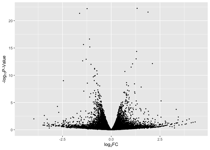
Basic Volcano Plot

data$label = if_else(rownames(data) %in% rownames(Top_Hits), rownames(data), "")
# basic plot
p1 <- ggplot(data, aes(log2FoldChange, -log(pvalue,10))) + # -log10 conversion
geom_point( size = 2/5) +
xlab(expression("log"[2]*"FC")) +
ylab(expression("-log"[10]*"P-Value")) +
xlim(-4.5, 4.5)
p1

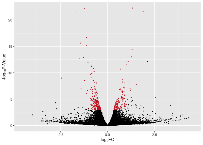
Basic Volcano Plot - Red Significant Genes

# basic plot with line + red for p < 0.05
p2 <- ggplot(data, aes(log2FoldChange, -log(pvalue,10))) + # -log10 conversion
geom_point(aes(color = Expression), size = 2/5) +
#geom_hline(yintercept= -log10(0.05), linetype="dashed", linewidth = .4) +
xlab(expression("log"[2]*"FC")) +
ylab(expression("-log"[10]*"P-Value")) +
scale_color_manual(values = c("firebrick3", "black", "firebrick3")) +
xlim(-4.5, 4.5) +
theme(legend.position = "none")
p2

# with labels for top 10 sig overall
library(ggrepel)
p3 <- ggplot(data, aes(log2FoldChange, -log(pvalue,10))) + # -log10 conversion
geom_point(aes(color = Expression), size = 2/5) +
# geom_hline(yintercept=-log10(0.05), linetype="dashed", linewidth = .4) +
xlab(expression("log"[2]*"FC")) +
ylab(expression("-log"[10]*"P-Value")) +
scale_color_manual(values = c("firebrick3", "black", "firebrick3")) +
xlim(-4.5, 4.5) +
theme(legend.position = "none") +
geom_text_repel(aes(label = label), size = 2.5)
p3

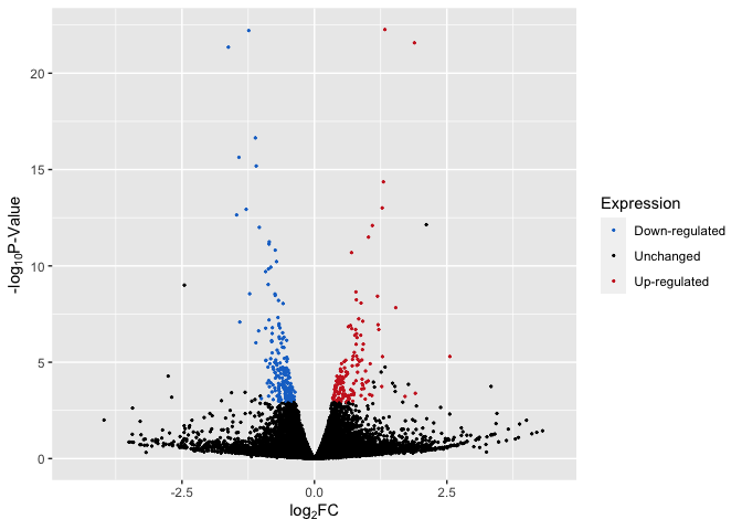
Up/Down Regulated Genes Identified

# plot with up/down
p4 <- ggplot(data, aes(log2FoldChange, -log(pvalue,10))) + # -log10 conversion
geom_point(aes(color = Expression), size = 2/5) +
#geom_hline(yintercept=-log10(0.05), linetype="dashed", linewidth = .4) +
xlab(expression("log"[2]*"FC")) +
ylab(expression("-log"[10]*"P-Value")) +
scale_color_manual(values = c("dodgerblue3", "black", "firebrick3")) +
xlim(-4.5, 4.5)
p4

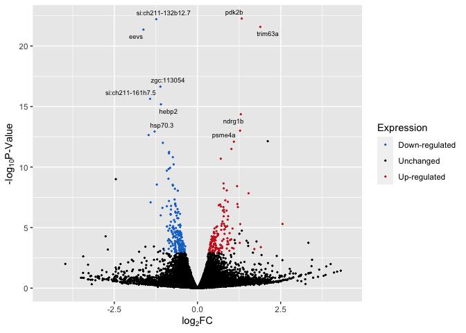
Up/Down Regulated Genes Identified and Labels

p5 <- ggplot(data, aes(log2FoldChange, -log(pvalue,10))) + # -log10 conversion
geom_point(aes(color = Expression), size = 2/5) +
# geom_hline(yintercept=-log10(0.05), linetype="dashed", linewidth = .4) +
xlab(expression("log"[2]*"FC")) +
ylab(expression("-log"[10]*"P-Value")) +
scale_color_manual(values = c("dodgerblue3", "black", "firebrick3")) +
xlim(-4.5, 4.5) +
geom_text_repel(aes(label = label), size = 2.5)
p5

Conclusion

Hope this tutorial was helpful! There are many other things that you can accomplish while analyzing differentially expressed genes. In fact, the next logical step would be to perform a gene enrichment analysis. Tutorial coming soon…